I’m sharing a small Python repo which I put together while figuring out how to build a Spacetime Gaussians renderer. This is a bare-bones stripped-down implementation that reproduces the math from the original paper and helped me wrap my head around the tricky parts – before I moved on to implementing a real-time renderer in Apple Metal.
If you want to skip to the code, see here >>
Motivation
High-performance renderers typically run on the GPU via CUDA or higher-level APIs such as OpenGL, WebGL, or WebGPU. The downside? GPU code is notoriously hard to debug. You can’t easily set breakpoints, print intermediate values, or step through execution the way you can on the CPU.
Gaussian splatting sits right at the intersection of traditional graphics pipelines and machine learning and it’s attracted interest from both communities. But for engineers coming from a Python/NumPy/PyTorch background, the challenge is often less about the math and more about the ecosystem of shader languages (GLSL, Metal, etc.), GPU APIs and the more rigid compiled structure of classic graphics pipelines.
Before translating into shader code, I started by prototyping in Python. This approach allowed me to:
- Focus on the core logic — the linear algebra, quaternion math, and projection geometry — without fighting shader syntax
- Use familiar Python tools to
print()intermediate matrices, plot 2D covariance ellipses with Matplotlib, and step through the code line by line. What’s opaque on the GPU becomes transparent on the CPU - Get real world values for unit testing
Repo Structure
On a very high-level, the repo simulates a long chain of mathemetiacal operations in a typical graphics pipeline:
Splat Data -> (Vertex Stage) -> 2D Ellipse Params -> (Rasterization Stage) -> Pixel Fragments -> (Fragment Stage) -> Final Pixel Color
The src directory contains the core logic, organised into modules that each represent a distinct part of the rendering process:
primitives.py: This file defines the fundamental data structures.Scene4D: A Structure of Arrays (SoA) that holds all scene data. For example, all splat positions are in one large NumPy array, all rotations in another, and so on. This is efficient for vectorised computation and for transferring data to a real GPU.Splat4D: An Array of Structures (AoS) where each object represents a single splat containing all its properties (xyz,rot,scale, etc.). This format is more intuitive for object-oriented processing.
io.py: This is the entry point for data. Theload_ply_4dfunction reads the.plyfiles, which store the trained Gaussian Splat data. It performs crucial initial transformations, such as applying activation functions, e.g.,np.exp()onscale, sigmoid onopacity.camera.py: A standard camera model that manages the view and projection matrices for transforming 3D world coordinates into 2D screen coordinates.utils.py: Contains helper functions. A key function isscene_to_objs, which converts the efficientScene4D(SoA) object into a list ofSplat4D(AoS) objects, preparing the data for per-splat processing in the vertex stage.render.py: This is the heart of the repo, containing the classes that simulate the main GPU pipeline stages:- Vertex Processing Stage
VertexProcessort, calculates its dynamic position, rotation, and scale. It then projects the resulting 3D Gaussian into camera space and computes the 2D covariance matrix that defines the ellipse’s shape on the screen. - Rasterization Stage
Rasterizer– takes the 2D ellipse from the vertex processor and determines which pixels on the screen it covers. It generates “fragment packets” for the next stage. - Fragment Processing Stage
FragmentProcessortakes the data for each pixel covered by a splat and calculates the final color and opacity, blending it correctly with what’s already on the screen. Framebuffer– after all primitives are processed, theframebuffer.bitmapholds the complete, rendered image for that frame, which is then displayed usingmatplotlib.pyplot.imshow.
- Vertex Processing Stage
The main rendering path _render_frame simulates a real GPU pipeline on the CPU.
Notes
“Gotcha” moments
Some of my most frustrating bugs weren’t in the math, but in the differing conventions between libraries, papers and platforms. I’m sharing my “gotcha” moments are where the real learning happened. They seem obvious and trivial in retrospect but it’s what tripped me along the way.
wxyzvs.xyzw– The original Gaussian Splatting paper, like many academic sources, uses thewxyz(scalar-first) notation for quaternions. However, SciPy’sspatial.transform.Rotationexpects thexyzw(scalar-last) format. Forgetting to re-order the components before passing them to the library doesn’t cause a crash; it just results in bizarre, nonsensical rotations that are a nightmare to debug. Here is a link to a helpful repo on the various quaternions conventions in different libraries and packages, https://github.com/clemense/quaternion-conventions.- Row-Major vs. Column-Major matrices – NumPy and SciPy default to row-major matrix order, which is standard in math. But graphics APIs like OpenGL and shader languages like GLSL expect matrices in column-major order. When you pass a flattened array to a shader, it fills the columns first. This means a standard NumPy matrix must be transposed before being sent to the GPU. Getting this wrong leads to completely scrambled transformations – squashed, sheared, and misplaced objects.
- Y-Up vs. Y-Down: In graphics OpenGL and WebGL use a “Y-Up” convention in their final coordinate space (as Unity and Houdini do, while Blender and Unreal Engine use Z-up). However, many 2D image libraries and some computer vision contexts use a “Y-Down” system where the origin is the top-left corner. This subtle difference impacts the signs of the Jacobian matrix
Jused for projecting the 3D covariance (link to original implementation by Inria). Using the wrong convention resulted in splats that were vertically flipped or distorted. I couldn’t initially catch the error in the simple toy examples and the final renders of real scenes looked eerily close but still wrong. - Covariance Transformation Order: The formula for the 3D covariance matrix
Σseems simple, but a subtle transposition can flip your splats. The standard textbook formula isΣ = R S² Rᵀ, which takes an axis-aligned ellipsoid (defined by the scaling matrixS) and rotates it byR. However, the SplaTV code which I was using as a reference calculates it asΣ = Rᵀ S² R. The two formulas,R S² RᵀandRᵀ S² R, produce ellipsoids with the exact same shape and size, but they are rotated in opposite directions becauseRandRᵀrepresent inverse rotations. If your pipeline is set up for the first formula (as mine was, following the paper), using the second will result in splats that are oriented incorrectly, as if reflected in a mirror. This bug is particularly tricky because the splats still look like plausible ellipsoids—they’re just not facing the right way. The entire transformation chain must be consistent, from how the rotationRis defined to how the covariance is constructed.
S², and rotate it by Rᵀ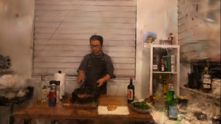
- The Sorting Saga: In a fundamental rule of rendering transparency, we sort sort objects from back to front to blend them correctly, i.e.
visible_splats.sort(reverse=False). However, I was wrongly sortingreverse=True. The confusing part? To compensate for the weird visuals, I had also flipped my camera to look from the opposite side (z=-5.0) instead of (z=5.0). The resulted was “close enough” to look plausible but was fundamentally broken. It was a classic case of two wrongs making a deceptive “right.” - Normalization: Quaternions must be normalised before feeding them into a rotation matrix formula. Otherwise, the rotation matrix doesn’t just rotate, it also incorrectly scales and skews the objects. My troubles started when I reused code that normalized the base rotation quaternion when it was first loaded. This is fine for 3D Gaussians, but in the case of Spacetime Gaussians, the logic adds a rotational offset to the base. The correct method is to add the base rotation and the time-dependent offset together first, and only then normalize the resulting quaternion once. This subtle logic error was only caught when I wrote specific unit tests to validate the rotation matrix output.
- The Need for Speed: Debugging a renderer is an iterative process. You tweak a camera parameter, change a line of math, and re-render to see the effect. This cycle is impossible when a single frame takes 10-20 minutes to render on one CPU core. So I had to implement some kind of multithreading (in my case with
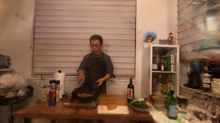
concurrent.futures) to bring bring the render times down to manageable 30-40 seconds, turning an impossible debug loop into a productive one. - The Power of Ground Truth: When you’re lost, having a single landmark you can trust is invaluable. For this project, the static 3D “Sleigh plush toy” scene was my first reference. By ensuring my 4D renderer could perfectly replicate this known-good 3D output, when things went wrong with animations, I could be confident the issue was in the new time-dependent logic, not the core projection and rasterisation.
Dual implementations
Some methods in the code have “dual” implementations – a “shader” model for clarity & portability and a “pythonic” model for performance & usability.
Methods with dual implementations include:
rasterize_primitive_naiveandrasterize_primitive_vectorizedshade_fragment_naiveandshade_fragments_vectorizedrender_frameandrender_frame_matplotlib
For example:
shade_fragment_naive(for loop-based) is conceptually identical to how a fragment shader on a GPU works – it’s executed independently and in parallel for every single pixel covered by a shape. The nested for loops in Python simulate this “one-program-per-pixel” model.
# Simplified logic from shade_fragment_naive
for x in range(x1, x2):
    for y in range(y1, y2):
        # ... calculate power, alpha for this single (x, y) pixel
# ... blend this single pixel into the framebuffershade_fragments_vectorized(NumPy-based) is a CPU-specific performance trick using NumPy arrays for the entire block of pixels because Pythonforloops are extremely slow.
# Simplified logic from shade_fragments_vectorized
# Create grids of coordinates for the entire bounding box
X_pixels, Y_pixels = np.meshgrid(...)
X_cam, Y_cam = np.meshgrid(...)Acknowledgements
Links to various resources which helped me.
Data
Community implementations
- antimatter15/splaTV | GitHub
- thomasantony/splat | GitHub
- huggingface/gsplat.js 4D splats example in JS Gaussian Splatting library | GitHub
- 3D Gaussian splatting for Three.js | GitHub
- A HDK/GLSL implementation of Gaussian Splatting in Houdini | GitHub
Math / conceptual walkthroughs
- Steps-by-step explanation of 3D splatting by Aria Lee on Medium
- Projecting 3D Gaussians to 2D math breakdown by xoft (in Korean)
- 4D Gaussian Splatting Explained by xoft (in Korean)
- Graphics Rendering Pipeline by Youngdo Lee
Reused code snippets
On compression & data representation
- Making Gaussian Splats smaller
- Making Gaussian Splats more smaller
- .splat universal format discussion #47
Leave a Reply